mtDNA: What your mama gave you!
March 9th, 2020
History Branch & Archives
833 N. Ocoee
Cleveland, TN 37311
Link to other presentations HERE
Updated 03/22/2020 – should be done in a few days.
Slide 01
This presentation is the ninth in a series of presentations that I have been asked to give for the Cleveland Bradley County Public Library History Branch & Archives. I’d like to thank Margot Still who runs the library for allowing me to do these.
Slide 02
So what is this presentation all about? The focus this month is to explore the third most popular DNA test and to compare it to the more popular ones to learn what mtDNA is and what kind of information the results of a mtDNA test will give us.
My professional background is 27+ years of computer training, course development, consulting, and I have a few published computer technology related books that I have worked on. I have taught over 350 different classes in my career. I primarily now teach companies on how to build a private and pubic clouds and use virtualization to extend their data center capabilities.
I have 45+ years of genealogy experience with the past 33 years using computer software to aid in my research. I have been on Ancestry.com since 2007.
Slide 03
Mitochondria are structures within cells that convert the energy from food into a form that cells can use. Each cell contains hundreds to thousands of mitochondria, which are located in the fluid that surrounds the nucleus (the cytoplasm).
Slide 04
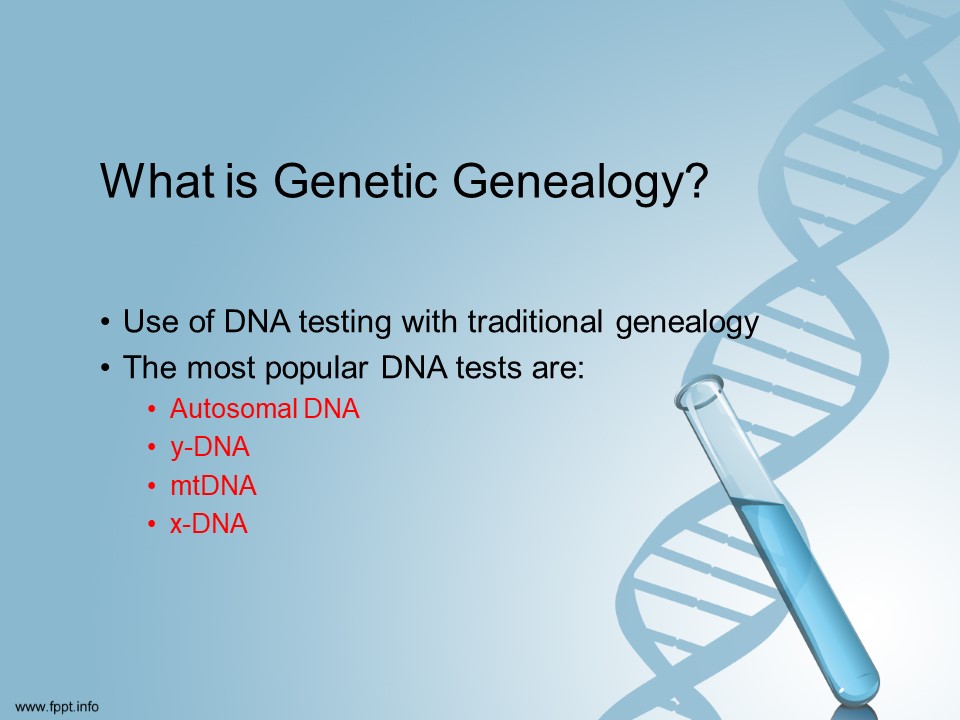
This presentation will review the purposes of the more popular Autosomal DNA and y-DNA tests to illustrate some of the similarities and differences in how each type of DNA works in regards to genealogical research.
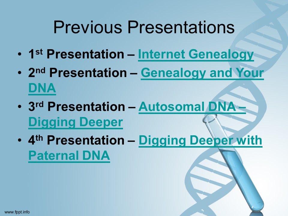
For more information see the presentation – Genealogy and Your DNA
Slide 05
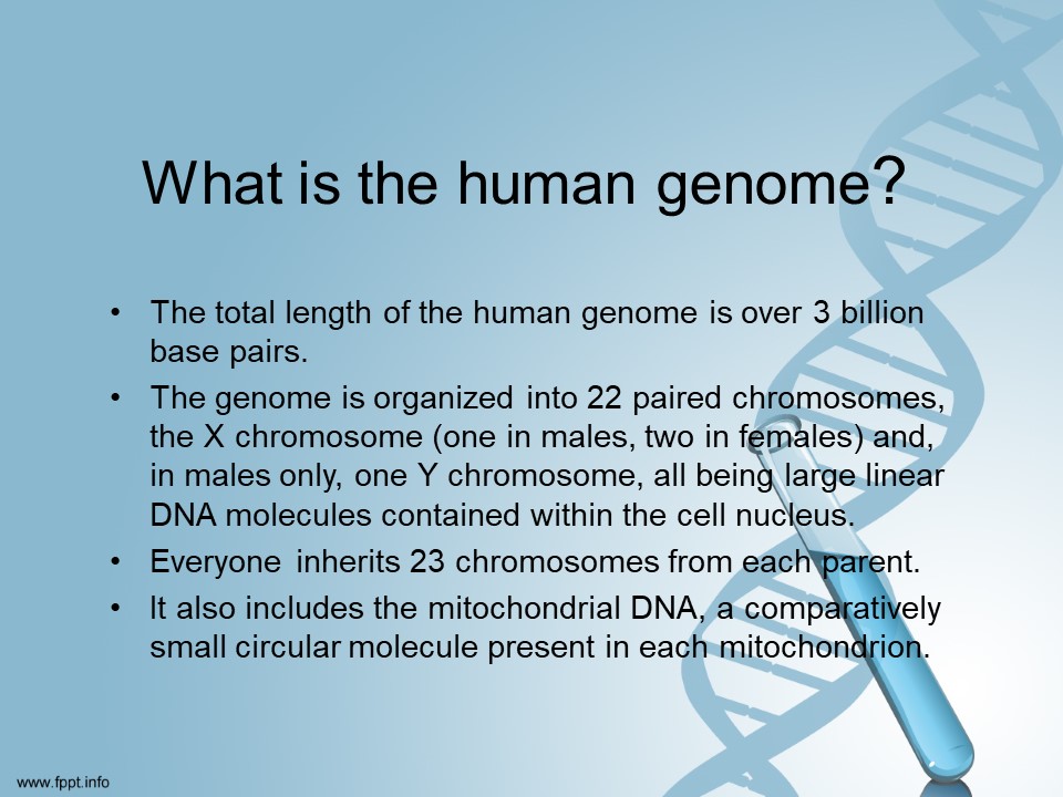
A basic understanding of the humane genome is important when deciding on what test(s) you should take. Each test provides help in determining relationships by comparing your test with someone else’s test to see if you share common DNA with them.
The slide covers the basics of what we have in regards to DNA in our cells.
Slide 06
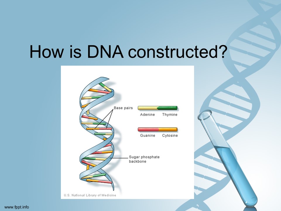
Base pairs are constructed using two complementary nucleotides. The four different nucleotides are shown in the image and are usually referred to their shortened name using the first letter A, T, G & C.
A & T can only bond together with each other and the same is true for G & C. They are connected to two strands of sugar phosphate to form the strands as shown in the image. Each chromosome labels the first base pair with a number all the way to its last base pair.
The base pairs can be in one of two orders: AT or TA and GC or CG. When identifying the sequence of base pairs they are referenced in that way.
See How DNA Works – https://science.howstuffworks.com/life/cellular-microscopic/dna1.htm
Photo courtesy U.S. National Library of Medicine
Slide 07
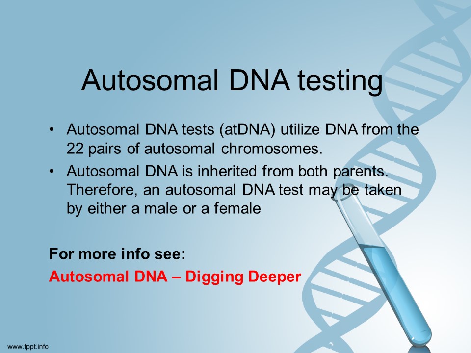
Autosomal DNA tests are the most popular test and the cheapest in cost. The advantage of taking this test is that you will be able to compare your test results with millions of other users. I like to say it is like throwing out a large fishing net. You are going to catch LOTS of relatives [for me it is over 3,000 people].
The value of any DNA test is only apparent if you compare it with someone else. The autosomal test looks at the first 22 sets of your chromosome at the base pair level and compares it to the person you are checking for matches. Having no common DNA does NOT necessarily mean you are not related. It is not uncommon for distant cousins like 5th or 6th cousins to not have any common DNA. The both have DNA from the same ancestor but not the SAME chunks of DNA.
For more info see – Autosomal DNA – Digging Deeper
Slide 08
Autosomal DNA tests are available for finding cousins and verifying relationships for genetic genealogy purposes are offered by 23andMe, AncestryDNA and Family Tree DNA (the Family Finder test).
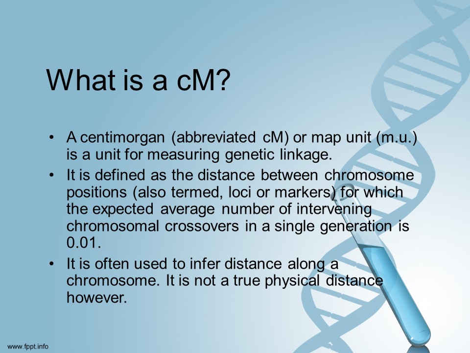
When you compare your autosomal DNA against someone else’s you will get a number of centimorgans from 0-3400 (approx.)
The higher the number the closer you are related.
| % shared | Total cM shared half-identical (or better) | Relationship | Notes |
|---|---|---|---|
| 100% (Method I)/50% (Method II) | 3400.00 | Identical twins (monozygotic twins) | Fully identical everywhere.[2] |
| 50% | 3400.00 | Parent/child | Half-identical everywhere |
| 50% (Method I)/37.5% (Method II) | 2550.00 | Full siblings | Half-identical on 50%/1700 cM and fully identical on a further 25%/850 cM. |
| 25% | 1700.00 | Grandparent/grandchild, aunt-or-uncle/niece-or-nephew, half-siblings | |
| 25% (Method I)/23.4375% (Method II) | 1593.75 | Double first cousins | Half-identical on 21.875%/1487.5 cM and fully identical on a further 1.5625%/106.25 cM |
| 12.5% | 850.00 | First cousins, great-grandparent/great-grandchild, great-uncle or aunt/great-nephew or niece, half-uncle or aunt/half-nephew or niece | |
| 6.25% | 425.00 | First cousins once removed, half first cousins, great-great-grandparent/great-great-grandchild, great-great-aunt/uncle, half great-aunt/uncle | |
| 6.25% | 425.00 | Double second cousins | |
| 3.125% | 212.50 | Second cousins, first cousins twice removed, half first cousin once removed, half great-great-aunt/uncle, great-great-great-grandparent/great-great-great-grandchild | |
| 1.563% | 106.25 | Second cousins once removed, half second cousins, first cousin three times removed, half first cousin twice removed | |
| 0.781% | 53.13 | Third cousins, second cousins twice removed | Up to 10% of third cousins will not share enough DNA to show up as match. See cousin statistics |
| 0.391% | 26.56 | Third cousins once removed | |
| 0.195% | 13.28 | Fourth cousins, third cousins twice removed | Up to 50% of fourth cousins will not share enough DNA to show up as match. See cousin statistics |
| 0.0977% | 6.64 | Fourth cousins once removed. third cousins three times removed | |
| 0.0488% | 3.32 | Fifth cousins | Only between 15% and 32% of fifth cousins will share enough DNA to show up as a match. See cousin statistics |
Notes to Table
- There is no variation between families in the parent/child or identical twins shared cM figures; beyond these immediate relationships, recombination results in random variation around the average figures above from one pair of individuals to another.
- When a grandchild is compared to a grandparent, the shared cM with the other grandparent on the same side is easily inferred. The grandchild gets all 3400cM of, say, his paternal autosomes from his father. If it is seen that 1600cM of this came from the paternal grandfather, then the other 1800cM must have come from the paternal grandmother. The initial estimate of 1700cM shared by grandchild and paternal grandmother can thus be updated to 1800cM when it has been ascertained that grandchild and paternal grandfather share only a below average 1600cM.
- When the subjects of the comparison descend from identical twin children of their most recent common ancestral couple, then the figures in the above table should be doubled.
- The expected % shared for a half-relationship will always be exactly half of the expected % shared for the corresponding full relationship.
- A similar method to that used for full siblings and for double first cousins can be used to compute expected shared percentages for any two subjects of comparison who are doubly related. However, the expected % shared for a double relationship can be slightly less than the sum of the expected % shared for the appropriate single relationships.
- If Jack is related to both of Jill’s parents, then Method I and Method II will give slightly different figures, as double cousins of this type are expected to be fully identical in some regions.
- If Jill is a more remote descendant of spouses who are both related to Jack, then Jill will clearly have inherited at most one of the two segments in regions where the child of those spouses was fully identical to Jack. This reduces Jack and Jill’s expected % shared slightly from the ballpark figure obtained by adding the expected % shared for the two relationships.
- For example, double second cousins, where the double relationship arises because at least one is related on both the paternal side and the maternal side to the other, are expected to share 3.125% (1/32) on each side, or 6.25% (1/16) in total, using Method I. Using Method II, a small adjustment must be made to allow for regions where they are fully identical (1/1024 or approximately 0.098%), so that they are expected to be half-identical or better on 63/1024 or approximately 6.152%.
- On the other hand, double second cousins who are children of double first cousins are expected to be half-identical on a quarter of the approximately 23.438% on which their parents are half-identical or better, in other words on approximately 5.859%.
For more info see – https://isogg.org/wiki/Autosomal_DNA_statistics
Slide 09
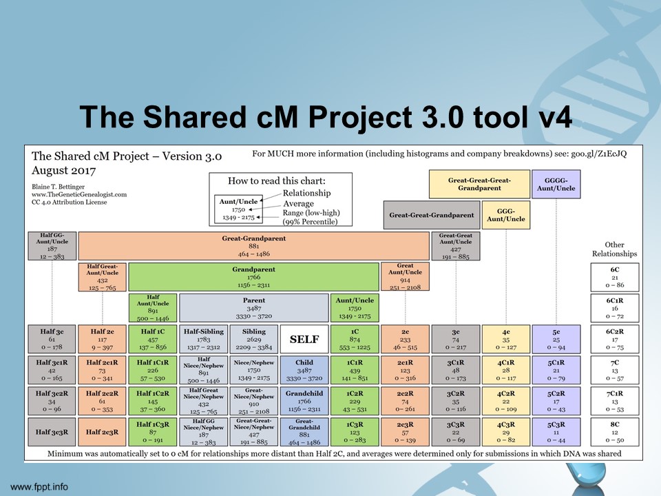
When comparing Autosomal DNA test results to someone else this is a good place to go if you are not sure how closely you are related.
The Shared cM Project 3.0 tool v4 – https://dnapainter.com/tools/sharedcmv4
This chart helps us determine what possible relationships we could have with a person. Let’s say you have a relative that you have 215 cMs in common. This chart shows that you could be a number of possible relationships based on that number. We can use that information to help us determine how many generations ago our MRCA lived. These numbers are based on observed numbers of known relatives. Notice that even with 0 common cMs you could still be related a number of different ways. The first number is the average for that type of relationship.
The tool allows you to enter the number of total cMs you have in common with the person you are comparing tests with and will tell you what type of relations will be possible. For instance if we enter 215 we will see this:
Relationship probabilities (based on stats from The DNA Geek)
- 49.29%Half GG-Aunt / Uncle 2C Half 1C1R 1C2R Half GG-Niece / Nephew
- 39.88%Half 2C 2C1R Half 1C2R 1C3R
- 6.04%Great-Great-Aunt / Uncle Half Great-Aunt / Uncle Half 1C 1C1R Half Great-Niece / Nephew Great-Great-Niece / Nephew
- 4.79%Half 1C3R † 3C Half 2C1R 2C2R
- ~ 0%** Half 2C2R
** this set of relationships is just within the threshold for 215cM, but has a zero probability in thednageek’s table of probabilities
† this relationship has a positive probability for 215cM in thednageek’s table of probabilities, but falls outside the bounds of the recorded cM range (99th percentile)
So the most likely relationship between you and your relative is either:
- Half GG-Aunt or Uncle
- 2nd Cousin
- Half 1C1R
- 1C2R
- Half GG-Niece / Nephew
I have a 2nd cousin who shares 215 cMs. Now we know how we are related but if you didn’t this could help you narrow down the possibilities.
Slide 10
In addition to helping you find new relatives autosomal DNA can help identify health related issues.
For more info see – Autosomal Recessive: Cystic Fibrosis, Sickle Cell Anemia, Tay-Sachs Disease
Slide 11
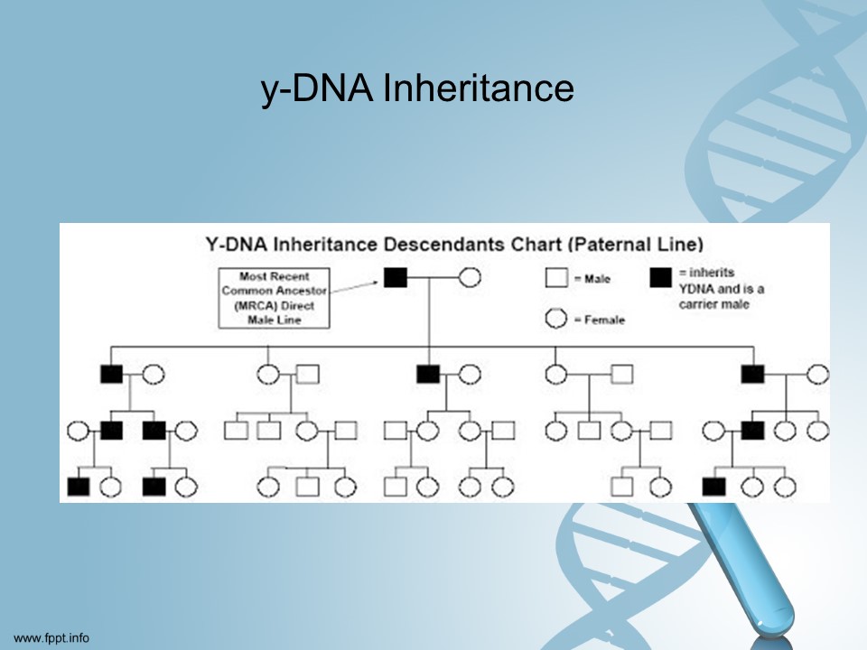
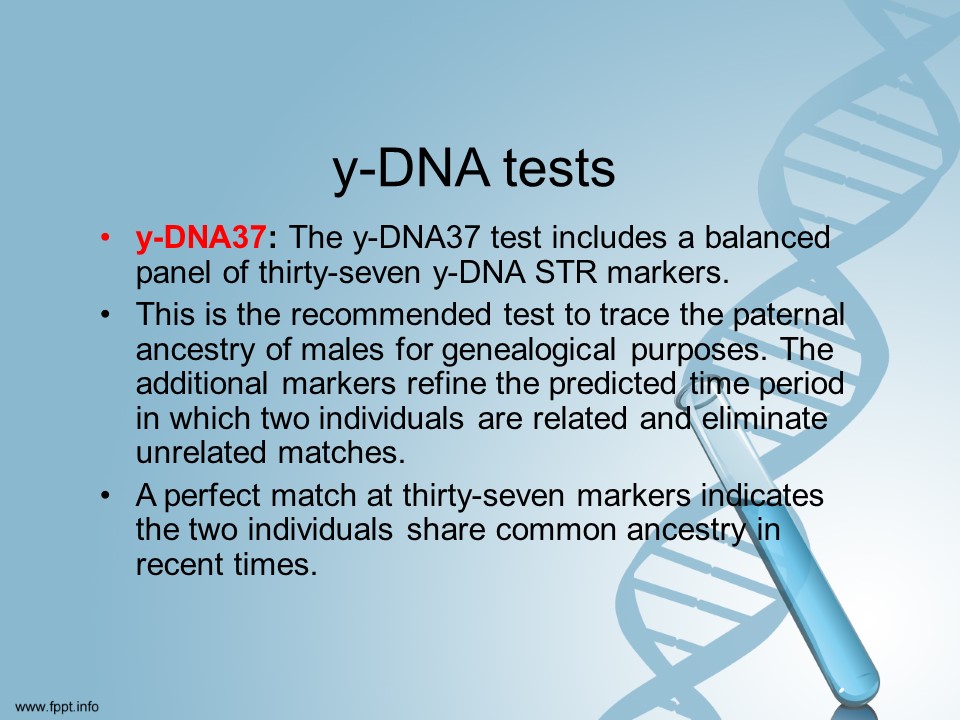
The second most popular DNA test is the y-DNA test. Only men can take this test.
Slide 12
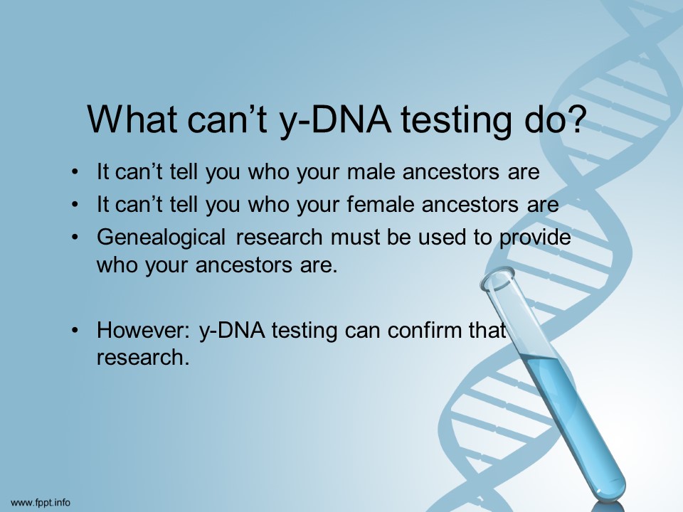
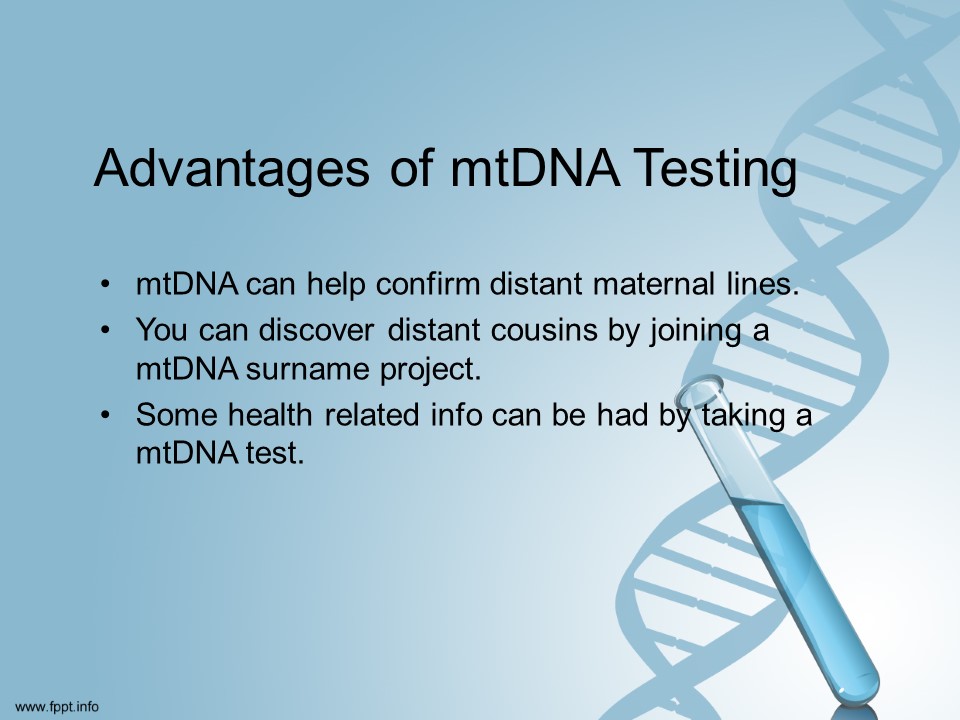
The y-DNA can only help you trace your birth surname. For male adoptees this is useful in helping you find your father’s direct ancestors.
Woman can benefit from this test by getting their father, brother or paternal uncle to take the test.
Slide 13
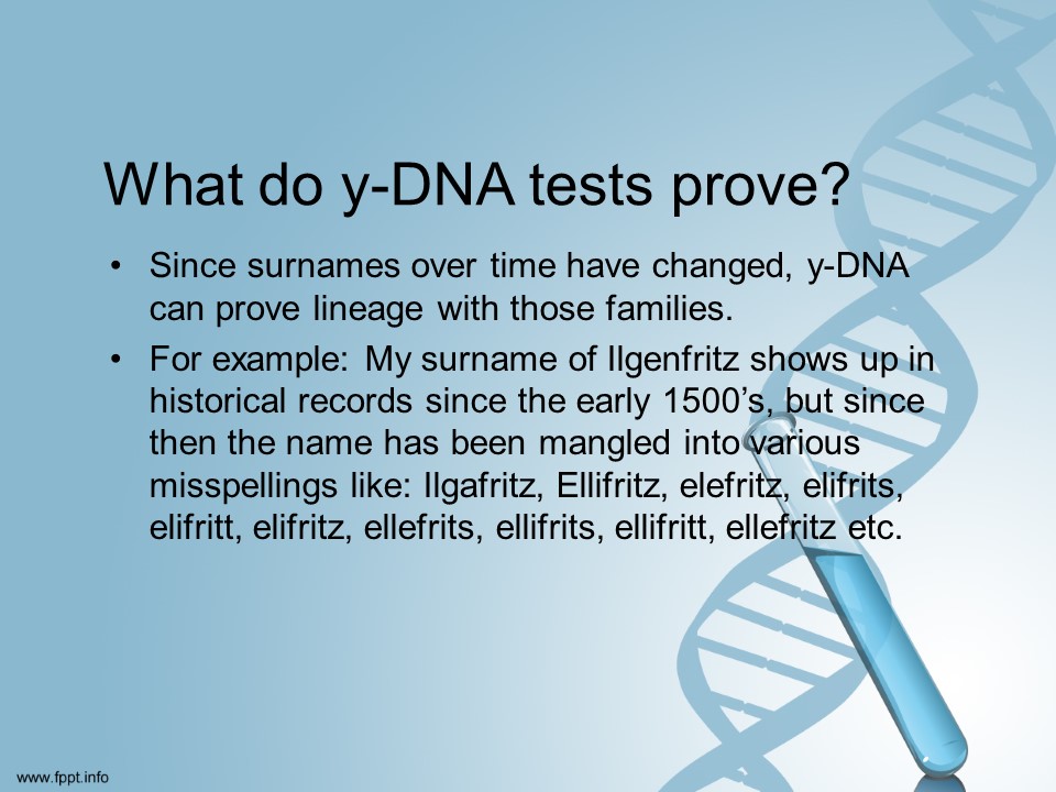
One of the challenging things to deal with when researching your family tree is misspelling of your surname in records. This test can help connect you with more distant ancestors than autosomal DNA since the y-DNA does not get diluted with each generation.
Slide 14
Will add notes from here onward tomorrow…stay tuned!
Slide 15
Slide 16
Slide 17
Slide 18
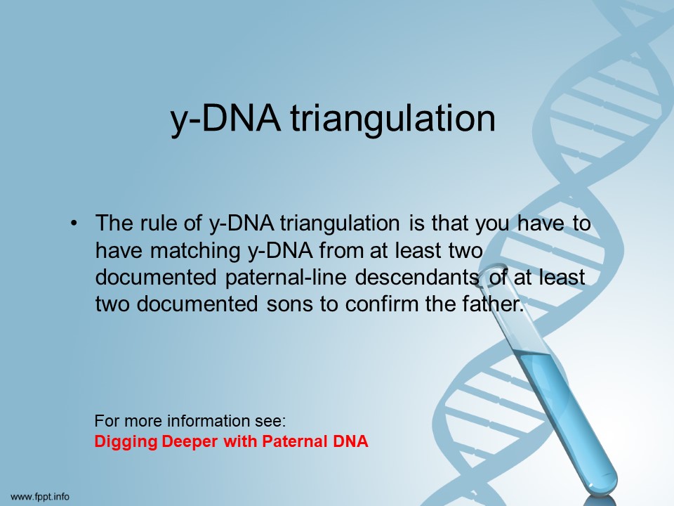
For more information see – Digging Deeper with Paternal DNA
Slide 19
Slide 20
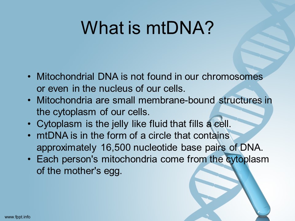
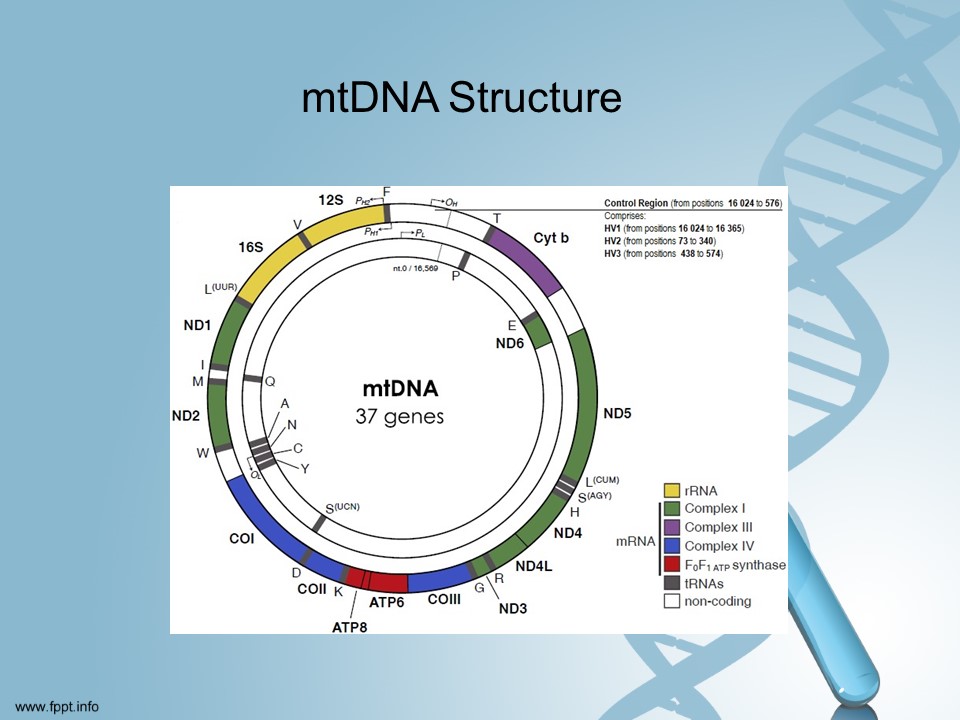
Each cell in the human body contains hundreds to thousands of mitochondria, which are located in the fluid that surrounds the nucleus (the cytoplasm) of each cell. Mitochondria are structures within cells which have the purpose of converting the energy from food into a form that cells can use.
Our mitochondrial DNA spans about 16,500 DNA building blocks (base pairs), representing a small fraction of the total DNA in cells.
Slide 21
Over the past few years scientists have been able to associate certain health conditions within the mitochondria.
The following conditions are associated with changes in the structure of mitochondrial DNA:
- Age-related hearing loss
- Cancers
- Cyclic vomiting syndrome
- Cytochrome c oxidase deficiency
- Kearns-Sayre syndrome
- Leber hereditary optic neuropathy
- Leigh syndrome
- Maternally inherited diabetes and deafness
- Mitochondrial complex III deficiency
- Mitochondrial encephalomyopathy, lactic acidosis, and stroke-like episodes
- Myoclonic epilepsy with ragged-red fibers
- Neuropathy, ataxia, and retinitis pigmentosa
- Nonsyndromic hearing loss
- Pearson marrow-pancreas syndrome
- Progressive external ophthalmoplegia
For more information see – https://ghr.nlm.nih.gov/mitochondrial-dna#conditions
Slide 22
Slide 23
Slide 24
Slide 25
Slide 26
Slide 27
Slide 28
To learn more about tools to aid in your mtDNA research go to – https://isogg.org/wiki/MtDNA_tools
Slide 29
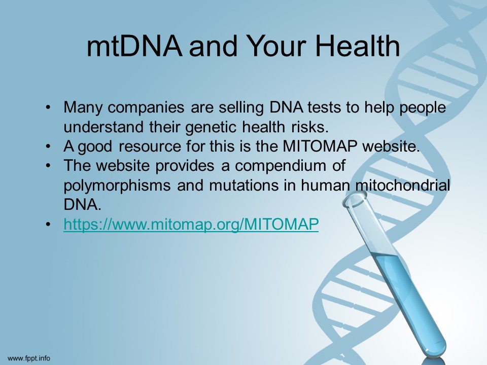
Mitomap website – https://www.mitomap.org/MITOMAP
Slide 30
Slide 31
Slide 32
Slide 33
Slide 34

Slide 35
Slide 36
Slide 37
Slide 38
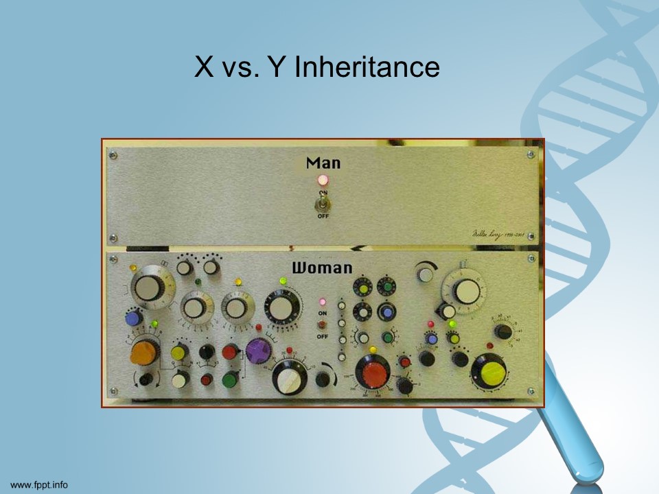
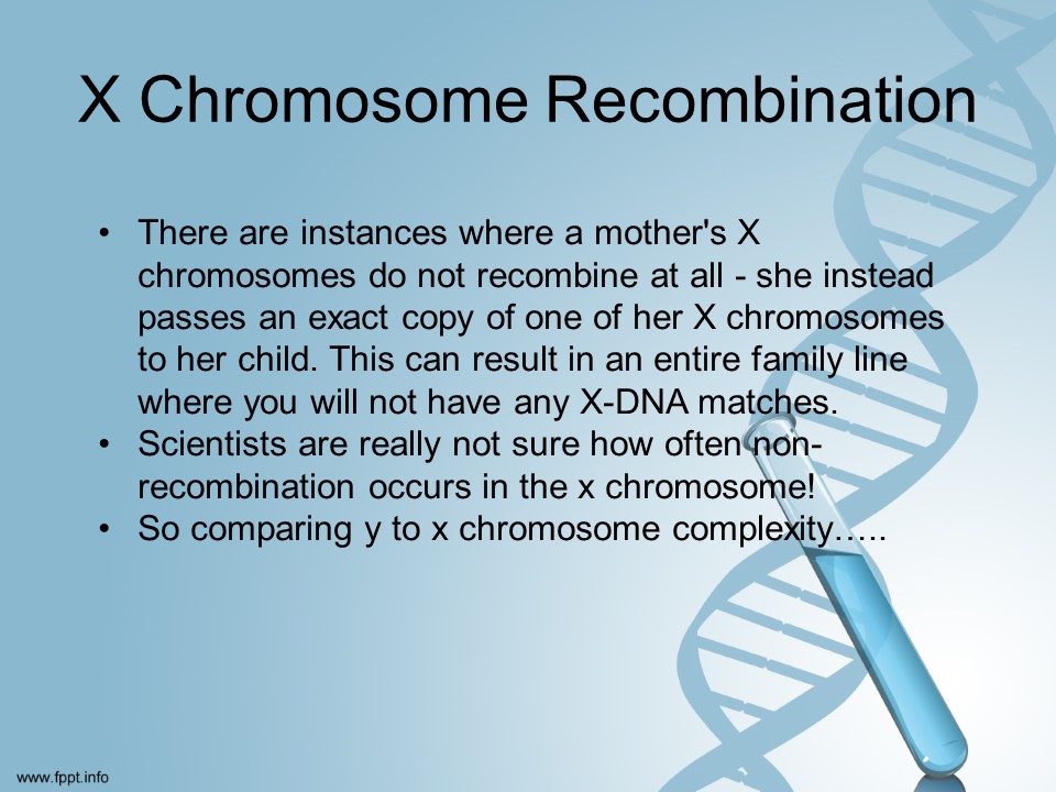
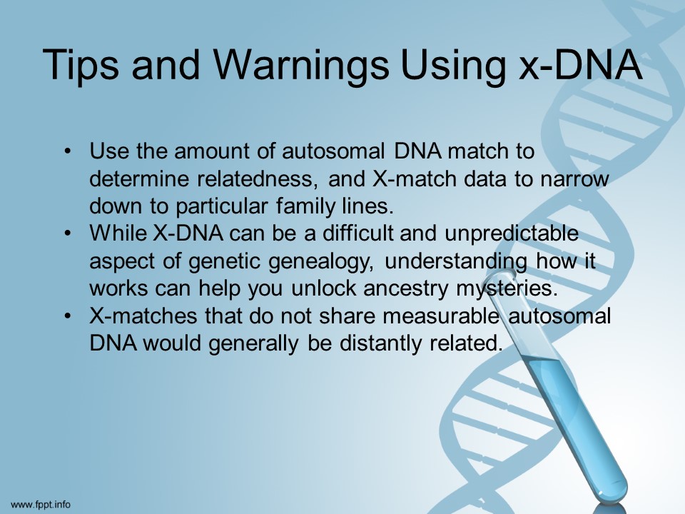
According to scientists [I promise I am not making this up!] yDNA is pretty easy to understand. xDNA is not entirely understood yet.
Slide 39
Slide 40
Slide 41
Slide 42
Slide 43
Link to other presentations HERE
Slide 44
Slide 45
Slide 46
Slide 47
If you are interested in any topics I haven’t covered, let me know and maybe I will use your suggestion for a future presentation.
Slide 48
End of Presentation